Using Solver in EXCEL

Using Solver for LP Problems

Obviously we can only solve very simple problems graphically. However, with any modern spread-sheet, linear optimization problems of any size can be solved very quickly. As a simple example, suppose a firm is producing 2 products and can sell them at prices . The firm wishes to solve the following problem in order to maximize revenue subject to two input constraints.

subject to the constraints

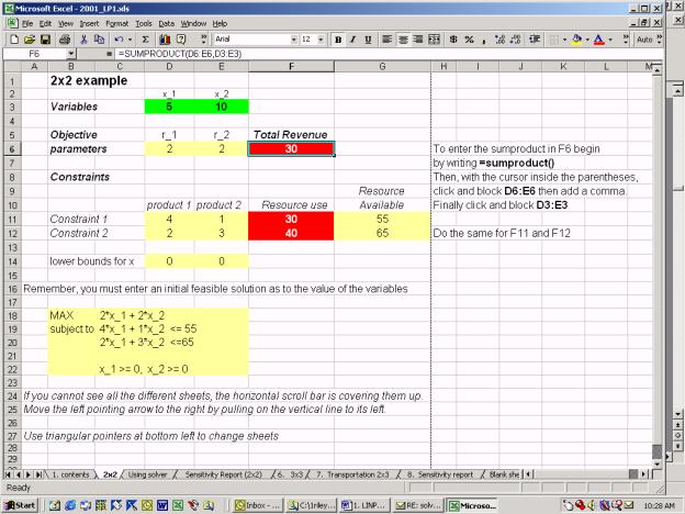
The picture below illustrates one way of setting up the spread-sheet. The first step is to list the variables and the unit payoffs. On the spread-sheet it is useful to use different colors for the variable cells, the data cells and the cells where there is a computation. We need to enter something in the variable cells as an initial guess.

Consider the Total Revenue cell, F6. It is the active cell in the picture. This is the vector product of the unit payoffs and the outputs . In Excel we write this as follows.

=sumproduct(D3:E3,D6:E6)

The next step is to write down the constraints. First we write down the input constraints. Again we use the vector product to get expressions for total resource use.Finally we write down any bounds for each variable. In this case there are lower bounds of zero.

We are now ready to use the program SOLVER. Set the cursor on the maximand (total revenue) then go to [Tools] and select [Solver].
Click to indicate that this is a maximization problem.
Go to the [Options] menu and click on [Linear Model]. Click on the [Changing Cells] then block out D3:E3 with the mouse. (Left click and hold while you block.)
Click on [Add] a Constraint. The following box will appear.

ADD CONSTRAINT
Cell reference			Constraint
		<= v
OK	Cancel	Add	Help

The constraint is that the block F11:F12 <= G11:G12. You need to move the cursor into the right blank space before blocking out each array.
Again click on [Add] to add the non-negativity constraints. Block out the variables D3:E3. Change the inequality to >= then in the right box block out D14:E14.
Click on [OK] This is what you should see.

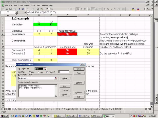
As long as your initial guess is feasible, go ahead and click on [Solve].

Try this yourself from scratch or download 2001_LP1.xls

With a little bit of luck you will have solved your first LP problem using Solver. The important point to note is that the method just described can be almost immediately extended to incorporate any number of variables and constraints.

If you get a solution, click on "Sensitivity Report" then choose O.K. This will add a new sheet with the results.

Adjustable Cells
			Final	Reduced	Objective	Allowable	Allowable
	Cell	Name	Value	Cost	Coefficient	Increase	Decrease
	$D$3	Variables x_1	10	0	2	6	0.67
	$E$3	Variables x_2	15	0	2	1	1.5

Constraints
			Final	Shadow	Constraint	Allowable	Allowable
	Cell	Name	Value	Price	R.H. Side	Increase	Decrease
	$F$11	Constraint 1 Resource use	55	0.2	55	75	33.33
	$F$12	Constraint 2 Resource use	65	0.6	65	100	37.5

Table C-4: Sensitivity Report

Consider Table C-4. In the “Adjustable Cells” section ("Changing Cells in earlier versions of EXCEL) there is an indication of how much each parameter of the objective function can change without affecting the solution . Thus as long as satisfies , the solution remains .Similarly, in the “Constraints” section, there is an indication of how much the supply of available resources can change without affecting the shadow prices . Thus as long as the resource availability levels remain in the “allowable” range, the same constraints will be binding.