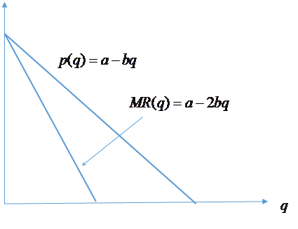
Marginal analysis and single variable calculus

        So much of economic analysis is about thinking on the margin in the pursuit of a more favorable outcome. Consider the choice of a firm that can produce a product at a cost of c per unit. The firm has some monopoly power. That is, it can raise its price without losing all of its customers and lower its price without being flooded with additional customers. For every price it sets, the market demand is

        As we shall see, it is helpful to “invert” this demand function and rewrite it as follows:

Written this way, the equation is called the firm’s demand price function. If the firm chooses to supply q units to the market then p(q) is the market clearing price.

Total revenue is then

Marginal analysis considers the rate at which one variable varies with another.  The graph of the revenue function, R(q), is depicted below.

Economists call the rate of change of revenue with output the marginal revenue, MR(q).  This is the incremental revenue when output increases from  to  divided by the increment in output  :

In some text books, marginal revenue is defined as the extra revenue from selling one more unit. But this typically not the case. A firm may be considering opening an additional plant that will increase capacity by 5%.  If current sales are 10,000 units per month, then the incremental output is 500 units per month. Of course one could describe this as “one unit of output capacity” but this is unnecessary.  The important point is that the increment in output is small.

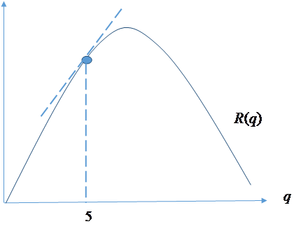
        In modelling economics we often ignore any indivisibility of a commodity and assume that a choice can be any real number in some interval.  We then define marginal revenue to be the limiting rate of change as the increment in output approaches zero.  In the figure below, as the increment approaches zero the rate of change (the steepness of the chord  becomes the steepness of the line touching the graph of the revenue function. 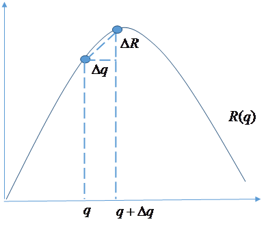This is the slope of the

the graph at a output level q.   For our quadratic example, we first compute the slope the chord depicted below, that is we compute    

If the slope of the chord has a limit as  approaches zero, then this limit is the slope of the graph at q.

      The new revenue is

The change in revenue is therefore

The slope of the chord is therefore

The marginal revenue at q is the limit as  approaches zero.

The demand price function and marginal revenue are depicted below. It is useful to remember that they both have the same intercept on the vertical axis and the marginal revenue curve is twice as steep.

In mathematical terms, marginal revenue is the derivative of the revenue function. We write the limit in one of the following ways:

Marginal profit is marginal revenue  marginal cost

If the right hand side is strictly positive, then the marginal profit is positive so the firm can increase its profit by increasing its output.

If the right hand side is strictly negative, then the marginal profit is positive so the firm can increase its profit by decreasing its output. Thus the profit-maximizing monopoly chooses the output level

From an economics perspective, this is not quite the whole story. Suppose that marginal profit is always negative.

           .

Note that this will be the case if and only if a < c. Then for any output q it is always more profitable to reduce output and so the profit-maximizing output is zero.

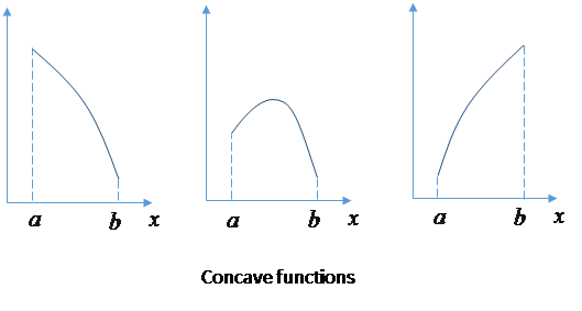
      In this introductory example, except for language, the analysis is essentially the same as in a basic calculus text.  Revenue and cost (and hence profit are defined for all positive real numbers, i.e. the interval  . For all  we showed that there is a single critical point (i.e. a point where the slope of the profit function is zero). We also showed that the slope was positive for all smaller  and negative for all larger . Thus the critical point is the profit-maximizing output.  With , the slope is negative for all output levels so the profit-maximizing output is zero.

Concave function

A function  with a slope, , that this decreasing over its domain  is called a concave function. In our example the profit function is concave. The graph of such a function can only have one of three possible shapes.  These are shown below. 

Thus if you find a critical point  satisfying  it must be the maximizing value.

         Economists often work with concave functions.

         For a concave function the slope,   is decreasing so the derivative of the slope (the second derivative,  ) is everywhere negative.  It is tempting to think that the second derivative must be strictly negative. This is almost true but not quite!  For example, suppose that  so that  and . Thus function has a maximum at  . The slope is everywhere decreasing but the second derivative not strictly negative at . 

Convex function

       Suppose a concave function is flipped upside down so that the slope is everywhere increasing. Mathematicians sometime say that such a function is concave upward. Economist always call such a function a convex function.